Preparing the Data for the Analysis

The rtweet package provides a simple way to pull tweets from the Twitter API. Additional packages listed below are also required.

library(rtweet)
library(vader)
library(tidyverse)
library(tidytext)
library(tidyr)
library(ggplot2)
library(dplyr)
library(knitr)
library(readxl)
library(igraph)
library(ggraph)

First, twitter handles for each US senator must be gathered. Luckily, a comprehensive list of all Twitter handles for members of the 116th Congress are available here. The accuracy of this list was cross-referenced here and corrections were made where necessary. Party affiliation was added to the database for comparison purposes between the Democrat and Republican parties. Two senators (Angus and Sanders) are officially listed as Independents, but were designated as Democrats for this analysis.

With the necessary data in hand, we load the dataframe into R and remove the “@” symbol from the list of handles.

X116th_Congress_Twitter_Handles <- read_excel("~/Documents/Projects/Twitter-Senators/116th-Congress-Twitter-Handles.xlsx")

senate <- X116th_Congress_Twitter_Handles

handles <-
  senate %>% select(Twitter_Handle, Party, State) %>% 
  mutate(Handle_stripped = tolower(str_remove_all(Twitter_Handle, "@")))

Next, we pass the senator handles through the get_timelines() command, where we pull a maximum of 1000 tweets per senator. The output of get_timelines() contains a number of different fields that we are not interested in for this analysis. For example, we are not interested in what senators retweet, but rather the tweets they create themselves. Accordingly, we select only a few relevant fields from the output.

#We save the get_timelines() output and then reload to save on future processing time
tmls <- get_timelines(handles$Handle_stripped, n = 1000) %>% 
  select(name, created_at, screen_name, text)

write.csv(tmls, ("~/Documents/Projects/Twitter-Senators/tmls.csv"))

tmls <- read.csv("~/Documents/Projects/Twitter-Senators/tmls.csv", header = TRUE)
tmls$created_at <- as.POSIXct(tmls$created_at)

We also only want tweets for the two months directly following Floyd’s death, so we use a date filter to restrict the dataset to tweets written between May 25th 2020 and July 25th 2020. Finally, tweets are messy data sources and need extensive tidying before we can use them for NLP analysis. Accordingly, we remove URLs, mentions, line breaks, special characters or emojis, ampersands, and any unnecessary blank space. We then join the dataset back onto our original table to attach the party and other desired information for each senator.

url_regex <- "http[s]?://(?:[a-zA-Z]|[0-9]|[$-_@.&+]|[!*\\(\\),]|(?:%[0-9a-fA-F][0-9a-fA-F]))+"

tmls_new <- 
  tmls %>% 
  dplyr::filter(created_at > '2020-05-24' & created_at < '2020-07-26') %>%
  mutate(text = str_remove_all(text, url_regex),
         text = str_remove_all(text, "#\\S+"),
         text = str_remove_all(text, "@\\S+"),
         text = str_remove_all(text, "\\n"),
         text = str_remove_all(text, '[\U{1f100}-\U{9f9FF}]'),
         text = str_remove_all(text, '&amp;'),
         text = str_remove_all(text, pattern = ' - '),
         text = str_remove_all(text, pattern = '[\u{2000}-\u{3000}]'),
         text = str_remove_all(text, pattern = '[^\x01-\x7F]'),
         text = str_squish(text),
         screen_name = tolower(screen_name)) %>% 
  left_join(handles, by = c('screen_name' = 'Handle_stripped')) %>%
  select(name, Party, State, created_at, text)

tmls_new$created_at <- as.POSIXct(tmls_new$created_at)

Next, since we are specifically interested in tweets having to do with policing, we select only those tweets that mention police and relevant variants of that word. We accomplish this by first constructing a variable that contains the words we are interested in, then applying the grep() function to create a dataframe with tweets containing at least one of the specific policing phrases.

police_var <- c("police","cop","cops","law enforcement","policing")
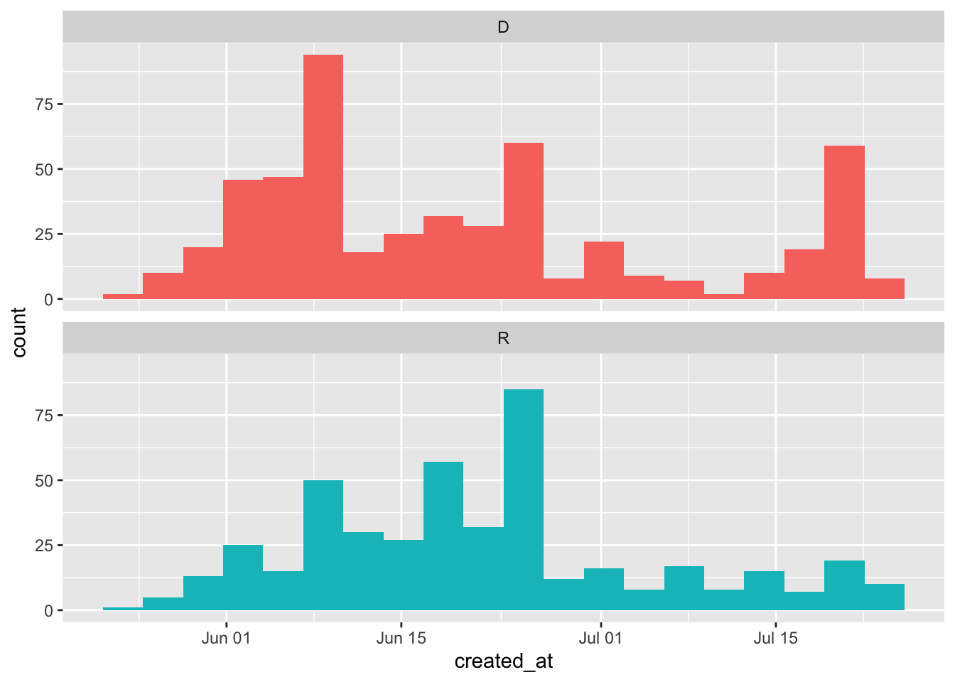
police_df <- tmls_new[grep(police_var, tmls_new$text),]

We can see how often tweets contain these words across the examined time period by plotting senators’ tweets grouped by party. As seen below, Democrat senators have more police-related tweets than Republican senators directly following Floyd’s death.

In the final steps of preprocessing we tokenize the words within the tweets and remove stopwords. Tokenizing is the process of identifying and separating each word from other words so that they are in a format that a machine can understand. Stopwords are extremely common words (e.g., “the”, “of”, “to”). Due to their high frequency of use they are not useful for analysis, and are typically removed in text mining.

police_words <- police_df %>%
  unnest_tokens(word, text) %>% 
  count(Party, word, sort = TRUE)

tidy_police <- anti_join(police_words, stop_words, 
                         by = "word")

Distributions, Frequencies, and Odds Ratios

To begin our analysis, we first calculate the number of times each word was used by a Republican or Democrat senator.

total_tidy_police <- tidy_police %>% 
  group_by(Party) %>% 
  summarize(total = sum(n))

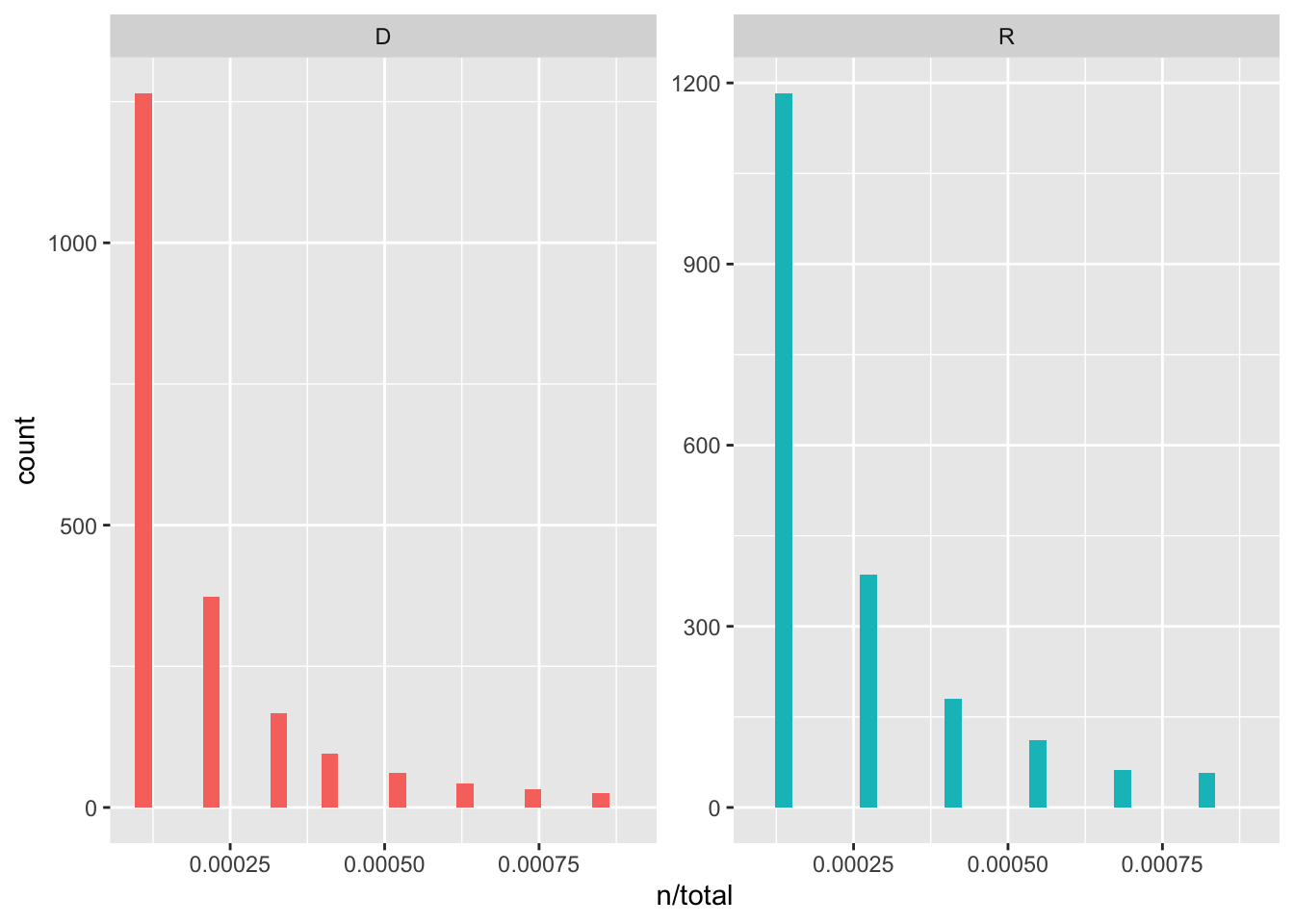
tidy_police <- left_join(tidy_police, total_tidy_police)

We then plot the distributions by party. What we observe are distributions that are typical in language. These long-tailed language distributions are referred to as Zipf’s law: the frequency with which a word appears is inversely proportional to its rank.

We next want to examine party differences between the frequency of word-use. That is, we want to see which words are being used frequently by both parties, and which words are being used with differing frequencies between parties. To do this, we first group by party and count how many times each senator used each word. Then we calculate a frequency for each senator and word.

tidy_police_frequency <- tidy_police %>% 
  group_by(Party) %>% 
  count(word, sort = TRUE) %>% 
  left_join(tidy_police %>% 
              group_by(Party) %>% 
              summarise(total = n())) %>%
  mutate(freq = n/total)

#We use spread() from tidyr to shape a dataframe that allows us to plot frequencies on the x- and y-axes of a plot.
tidy_police_frequency <- tidy_police_frequency %>% 
  select(Party, word, freq) %>% 
  spread(Party, freq) %>%
  arrange(D, R)

We now plot our word frequencies, grouped by party. Words near the red line are used with equal frequency by Republicans and Democrats, while words away from the line are used more by one party compared to the other.

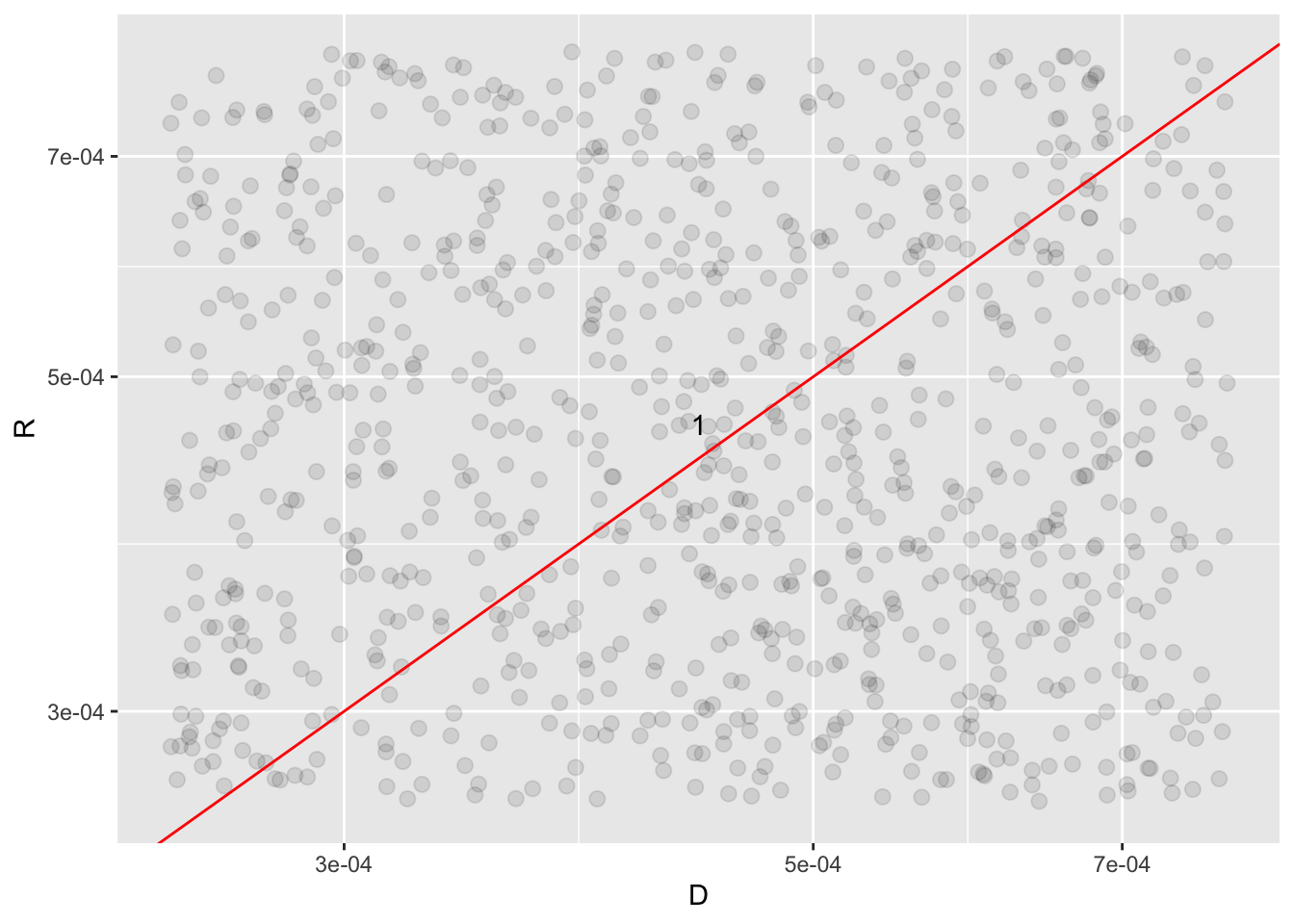
From the above plot we can see that Democrats use words such as “racism”, “black”, and “excessive” much more frequently than Republicans. While Republicans use words such as “safe”, “security”, and “crime” much more frequently than Democrats.

We can get an even clearer picture of the words used most frequently by each party by finding which words are more or less likely to come from each senator’s account using the log odds ratio. We then plot the top 15 most distinctive words from each party’s twitter statements.

police_ratios <- tidy_police %>%
  count(word, Party) %>%
  group_by(word) %>%
  filter(sum(n) >= 10) %>%     #We evaluate words only used more than 10 times.
  ungroup() %>%
  spread(Party, n, fill = 0) %>%
  mutate_if(is.numeric, list(~(. + 1) / (sum(.) + 1))) %>%
  mutate(logratio = log(D / R)) %>%
  arrange(desc(logratio))

police_ratios %>% 
  arrange(abs(logratio))

## # A tibble: 309 x 4
##    word             D       R logratio
##    <chr>        <dbl>   <dbl>    <dbl>
##  1 voted      0.00149 0.00150 -0.00963
##  2 reforms    0.00512 0.00525 -0.0256 
##  3 violence   0.00628 0.00650 -0.0356 
##  4 abuse      0.00182 0.00175  0.0369 
##  5 introduced 0.00182 0.00175  0.0369 
##  6 protests   0.00182 0.00175  0.0369 
##  7 america    0.00495 0.00475  0.0417 
##  8 vote       0.00314 0.00300  0.0444 
##  9 african    0.00132 0.00125  0.0549 
## 10 death      0.00330 0.00350 -0.0584 
## # … with 299 more rows

Bigrams

So far, we have been evaluating each party’s rhetoric regarding policing using single words. However, we can also tokenize senators’ tweets into consecutive words, called n-grams. By seeing how word X is followed by word Y, we can gain better insight into the meaning within senators’ tweets.

#Extract bigrams
police_bigrams <- 
  police_df %>% 
  unnest_tokens(bigram, text, token = "ngrams", n = 2)

#Separate the words in the bigrams for network analysis
police_bigrams_separated <- police_bigrams %>%
  separate(bigram, c("word1", "word2"), sep = " ")

#Remove stopwords
police_bigrams_filtered <- police_bigrams_separated %>%
  filter(!word1 %in% stop_words$word) %>%
  filter(!word2 %in% stop_words$word)

#Calculate a bigram count
police_bigram_counts <- police_bigrams_filtered %>% 
  count(word1, word2, sort = TRUE)

#Filter for only bigram combinations that occur greater than 10 times.
police_bigram_graph <- police_bigram_counts %>%
  filter(n > 10) %>%
  graph_from_data_frame()

#First, we rejoin stopword filtered bigrams
police_bigrams_united <- police_bigrams_filtered %>%
  unite(bigram, word1, word2, sep = " ")

police_bigram_tf_idf <- police_bigrams_united %>%
  count(Party, bigram) %>%
  bind_tf_idf(bigram, Party, n) %>%
  arrange(desc(tf_idf))

Sentiment Analysis

Finally, we can examine differences between the two parties with sentiment analysis. When individuals read text, they use their understanding of the emotional intent of words to infer whether a section of text has a positive or negative valence. We can use text mining sentiment analysis tools to extract the emotional content of senators’ tweets. We use the VADER package, since the sentiment scoring rules it uses were established from social media blogs.

#First, we create an error catcher to return NA for a tweet that VADER cannot process.
vader_compound <- function(x) {
  y <- tryCatch(tail(get_vader(x),5)[1], error = function(e) NA)
  return(y)
}

#VADER calculates sentiment scores.
vader_scores <-
  police_df %>% 
  mutate(vader_scores = as.numeric(sapply(text, vader_compound )))

Now we can calculate the 10 most positive senators on Twitter, when talking about policing.

vader_mps <-
  vader_scores %>%
  group_by(name, Party) %>%
  summarise(mean_score  = mean(vader_scores, na.rm = TRUE), .groups = 'drop') %>%
  top_n(10, mean_score) %>%
  arrange(desc(mean_score))

vader_mps

## # A tibble: 10 x 3
##    name                          Party mean_score
##    <chr>                         <chr>      <dbl>
##  1 Senator Jerry Moran           R          0.964
##  2 Senator Deb Fischer           R          0.944
##  3 Sen. Susan Collins            R          0.866
##  4 Jim Risch                     R          0.859
##  5 Senator John Hoeven           R          0.844
##  6 Senator Pat Roberts           R          0.836
##  7 Richard Shelby                R          0.795
##  8 Senator Thom Tillis           R          0.755
##  9 U.S. Senator Cindy Hyde-Smith R          0.735
## 10 Senator Gary Peters           D          0.708

Interestingly, the top 9 most positive senators, when tweeting about policing, are Republicans. We can compare sentiment across parties to see if this observation holds true across all senators.

vader_temp <- vader_scores %>% dplyr::filter(Party %in% c('D', 'R'))

As can be seen above, across all senators, Democrats express more negative sentiment toward policing than Republicans.

Finally, we can see how party sentiment scores developed across the two months following Floyd’s death while in police custody.

vader_time <- 
  vader_temp %>% 
  mutate(Date = as.Date(created_at)) %>% 
  group_by(Party, Date) %>% 
  summarise(mean_score = mean(vader_scores, na.rm = TRUE))

When examining sentiment by party across time, a more nuanced story emerges. Immediately following Floyd’s death, Republican senators spoke about policing in much more positive terms than Democrat senators. However, across time, Republican senators’ sentiment became more and more negative, until ultimately at the end of June 2020, aligning with negative Democrat senator sentiment.

Takeaways

This analysis has shown distinct differences between Republican and Democrat senators’ rhetorical response to policing in the months following George Floyd’s death. In an increasingly polarized political environment, perhaps this isn’t too surprising. Regardless, as demonstrated here, we can see that text mining methods allow us to better understand political leader rhetoric surrounding the issues of policing in the US.